
carloscastilla - Fotolia
Follow these examples to use CloudWatch Logs Insights
CloudWatch Logs Insights helps organizations gain insights from a deluge of log data on applications and services. Learn how to implement key features.

Developers and ops teams can use Amazon CloudWatch Logs to debug applications on AWS, but log analysis can quickly become complicated. AWS CloudWatch Logs Insights can improve that process.
A search through log files and plotting statistics is the most basic way to diagnose issues and dig into potential application issues. Logs are also the first place IT teams look when there's an attack on an application. But there is a downside. Logs have been notoriously expensive to parse at scale. They often take a significant amount of time to sort through for useful information. This is especially true if the logs come from multiple sources, some of which -- such as an API gateway -- might be out of your control.
Developers can use CloudWatch Logs to set up analytics based on preconfigured queries. Alternatively, they can use CloudWatch Logs Insights to dig into logs that are already stored, to plot statistics. While CloudWatch Logs Insights can improve log analytics, the tool has some limitations. Learn about its main querying and chart-building features, as well as helpful tips for filtering and use, with plenty of examples below.
Core features of CloudWatch Logs Insights
To understand the utility of CloudWatch Logs Insights, let's start with an example scenario. You log how long it takes to deliver a file via FTP servers. You track the time from when the file is received on the organization's FTP servers to when it's delivered to the customer's FTP servers. These logs come from legacy systems that run on EC2 instances and output JSON-formatted logs to CloudWatch Logs. While these logs show how long a specific file takes to deliver, they cannot reveal an average delivery time from the company's FTP server to the customer's. With CloudWatch Logs Insights, AWS users can quickly build ad hoc queries to do such things as plot the average file delivery time. Therefore, they can avoid using a third-party log aggregation tool. Queries set up through CloudWatch Logs Insights can reveal sundry information about application operations and performance.
As another example, in my role at a content syndication firm, I can see how many stories of each publication type we've received in the last hour if I enter the simple query shown in Figure 1.
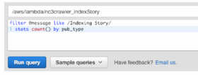
This works because AWS already parses a pub_type field since it's sent in via a JSON format. It's also possible to parse a message that's provided as text. For example, the following query parses a log line that includes a story ID, which comprises the publisher ID followed by a publication ID and a unique ID. I can parse this line using the parse command and then graph how many stories per publication were received, grouping the results into 30-minute intervals.
filter @message like /STORY Created/
| parse 'STORY Created *-*-* *' as publisher, publication, story_id, external_id
| stats count() by bin(30m), publication
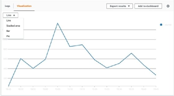
This results in a list of events that can be exported to a spreadsheet tool such as Microsoft Excel and graphed. At the time of publication, CloudWatch Logs Insights does not support graphing more than one dimension on a time series graph. You can filter for a specific publisher or publication in this example, but can't plot all of them on one graph. I can use the Visualization tab if I remove the , publication modifier at the end of the parsing command sequence.
You can also add these charts to CloudWatch dashboards to identify key metrics at a glance in the future. These dashboards can be shared with other members of DevOps teams, or even shared publicly to give non-AWS users insights into behind-the-scene metrics on how a system is operating.
CloudWatch Logs Insights makes it possible to perform complex math, such as plotting differences between two timestamps, right within the CloudWatch Logs platform rather than via a separate tool. Let's use another example from content syndication that you can extrapolate to apply in other fields with other products. The following example queries how long it takes to receive an article after it has published, by publication type, averaged over 30 minutes.
filter @message like /Indexing Story/
| stats avg(received_at - date) by bin(30m), pub_type
With a different setup, the filter command can track a specific publication and graph that information over time.
filter @message like /Indexing Story/
| filter publication = "XXXXXX"
| stats avg(received_at - date) by bin(30m)
Or, identify any publications that have a number of stories delayed more than 15 minutes.
filter @message like /Indexing Story/
| fields (received_at - date) as delay_time, @message
| filter delay_time > 90000
| stats count() as delayed_stories by publication
| sort delayed_stories desc
CloudWatch Logs Insights users can pipe commands, which means they send output from one command for further processing by another. For example, you can use the output of the fields command to filter on a newly created field, and the output of the stats command to sort by publications with the highest number of delayed stories first.
Structuring logs
CloudWatch Logs Insights allows parsing ad hoc text strings into structured data. However, it's often better to output relevant log metrics into pre-parsed JSON text strings. For example, an application is logging information about a request. Rather than outputting a line like GET /foo 200, consider instead outputting the code below.
{ "method": "GET", "path": "/foo", "status": 200 }
This text string is formatted so that CloudWatch Logs Insights can pre-parse this message. Rather than having to filter and then parse this specific message, the query can simply look for those specific fields.
stats count() by status, method, path
Additional visualization types
As part of CloudWatch Logs Insights, AWS users may also produce basic bar, stacked area and pie charts from metrics. Consider using these charts in CloudWatch dashboards to identify information such as the average HTTP status response code. For example, from an AWS HTTP API Gateway log, use the following query to plot status code responses.
stats count() by status
Select the Visualization tab and choose Pie.
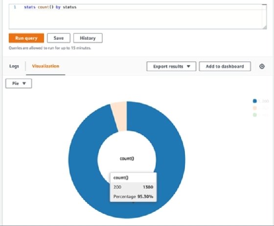
In the above example, I can see that the majority -- about 95% -- of responses for this particular API endpoint are status code 200 for OK, meaning the request succeeded.
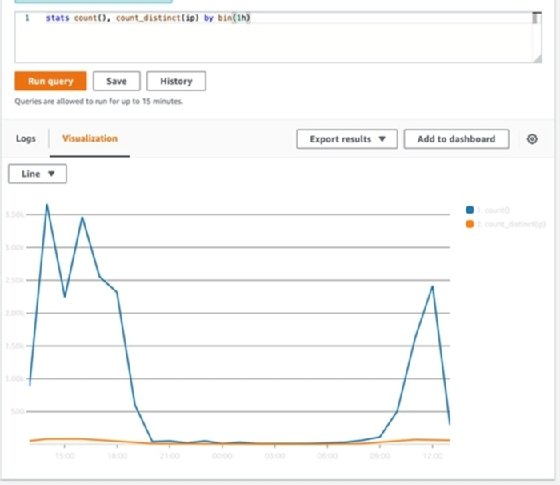
To plot multiple metrics over a single dimension, such as time, separate them with a comma. For example, to see both the number of requests and the number of unique IP addresses making those requests over a timeline, use the code below.
stats count(), count_distinct(ip) by bin(1h)
Visualizing Lambda cold start delays
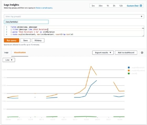
CloudWatch Logs Insights can parse AWS Lambda logs to identify the frequency and severity of Lambda cold start delays. Since AWS Lambda logs a line that indicates the total "Init Delay," first filter for messages that include a cold start, and then summarize those statistics.
fields @timestamp, @message
| filter @message like /Init Duration/
| parse 'Init Duration: * ms' as initDuration
| stats avg(initDuration), max(initDuration), count() by bin(1d)
Graphed onto a line chart, this information illustrates the average and maximum delay (in milliseconds) that a cold start creates, as well as the total number of cold starts that occurred on a specific day.
Absolute vs. relative time filtering
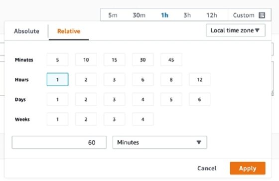
CloudWatch Logs Insights offers two ways to filter data by time: absolute and relative. Relative time filtering can identify recent activity. Relative filtering is beneficial for dashboard graphs, as the start and end date will always adjust relative to the current date on the dashboard. The default filtering option offers ranges for minutes, hours, days and weeks.
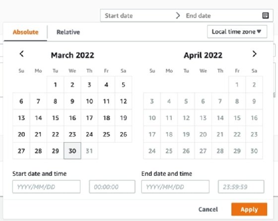
Alternatively, the absolute filtering option shows a specific point in time. Use it to track down issues, such as an anomalous amount of activity during certain hours. When AWS users define Start date and End date for this filter, they can see all data from between those two dates.
What CloudWatch Logs is still missing
For performance reasons, the CloudWatch Logs agents are configured by default to only send logs once every five seconds. This interval, combined with slow indexing times, can delay the appearance of a log, sometimes up to a few minutes, in CloudWatch Logs. This delay can be detrimental to the development process, if a developer has to wait from issuing a request to seeing the related logs in the back end. Users can configure the default five-second delay for CloudWatch agents, but only in certain situations. For example, you cannot change this on Lambda, but can change it for EC2 instances logging to CloudWatch Logs.
CloudWatch Log Insights may be enough log aggregation and analysis for most AWS users. With the continual improvements and additions to the service, expect a fully featured system built directly into the cloud provider's platform. Direct integration with the company's services like Amazon API Gateway is also a benefit, giving one spot for all logs generated throughout an application.